
CancerFit: Quickstart Tutorial
Address correspondence to: Lohith Kini ( )
)
Step 1: Download Mortality Data
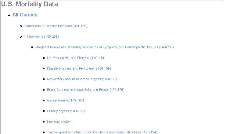
- Go to http://epidemiology.mit.edu/Mortality/mortality.html and choose the disease under study.
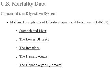
- As an example, you will run a CancerFit analysis on Pancreatic Cancer Mortality Data for European American Females. To download the data for Pancreatic Cancer, choose Digestive organs and Peritoneum (150-159) under Malignant Neoplasms, including Neoplasms of Lymphatic and Hematopoietic Tissues (140-208) and then choose The Lower GI Tract (http://epidemiology.mit.edu/Mortality/CancerofthelowerGITract.html)
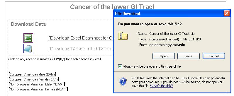
- Download and save the zip file containing text files by clicking on the [Download TAB-delimited TXT files for all plots] link.
Step 2: Start CancerFit in MATLAB
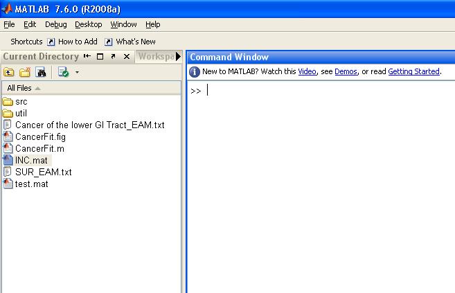
- Start MATLAB and go to the directory containing CancerFit.
- Run CancerFit by typing "CancerFit" at the command line and hit Enter.
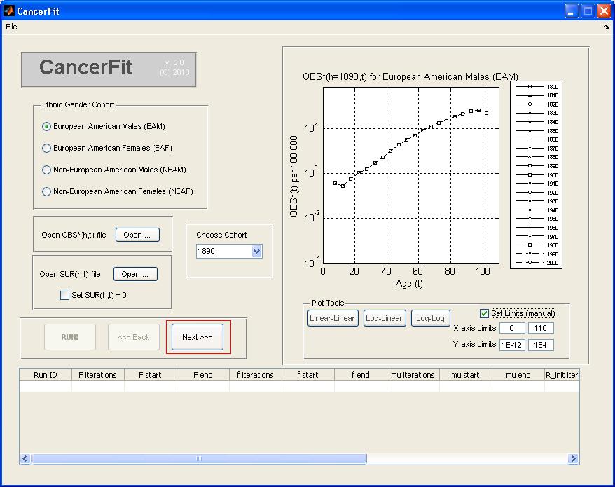
Step 3: Initialize a CancerFit Analysis
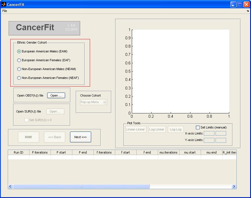
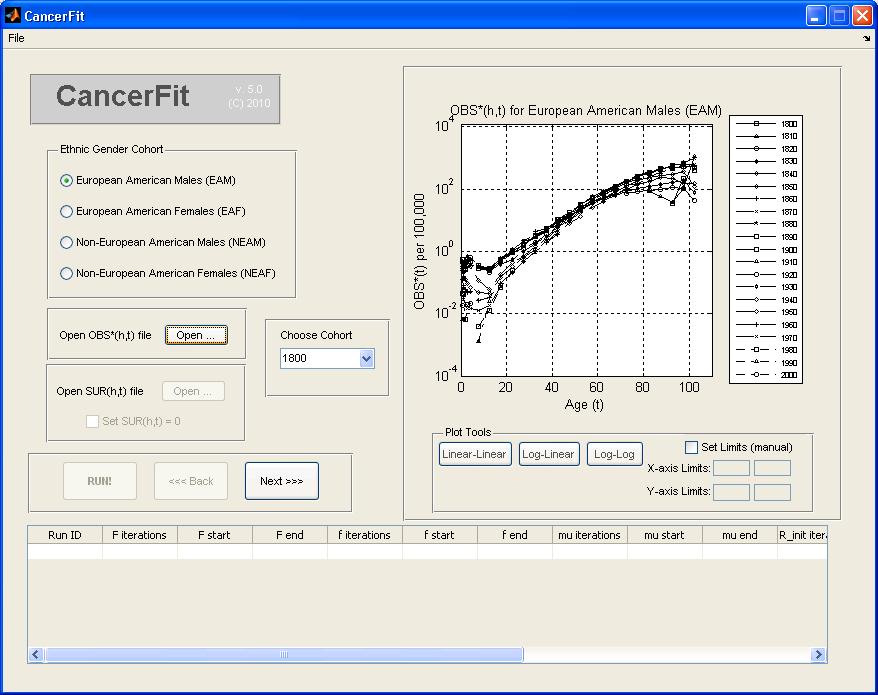
- Choose the Ethnic Gender of the mortality data to be analyzed. Choose European American Males (EAM) for this example.
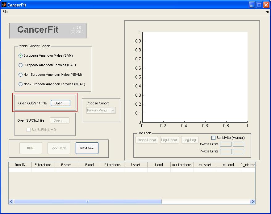
- Click "Open ..." button to open the TXT OBS*(h,t) file.
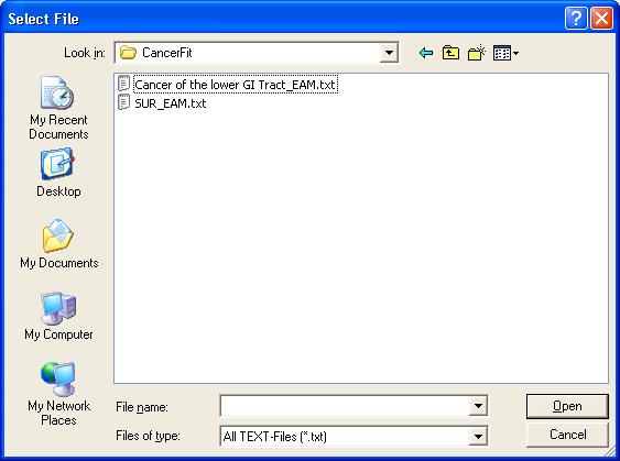
- Navigate to the location of the txt files extracted from the zip file for the disease being analyzed.
- Choose the txt file with Mortality data for the ethnic gender you chose before. For instance, to analyze Mortality Data for European American Males (EAM), pick the file named "Cancer of the lower GI Tract_EAM.txt" and click Open. The graph plot on the right will show mortality curves for all birth cohorts.
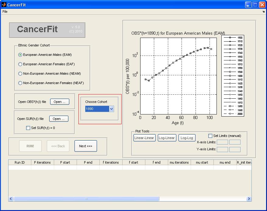
- Choose the birth Cohort (h) under the list "Choose Cohort". For this example, pick 1890 to analyze the birth cohort of the 1890s decade. The graph plot on the right will show the OBS*(h=1890s,t) mortality curve.
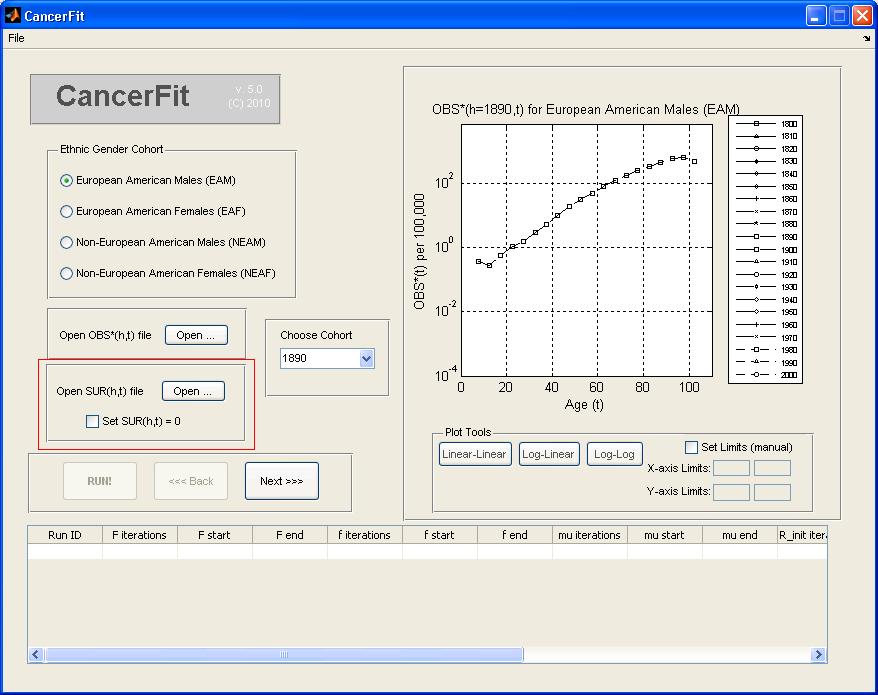
- Choose the SUR(h,t) file by clicking "Open ..." or choose to set SUR(h,t) = 0 such that CAL(h,t) = OBS*(h,t). An example SUR(h,t) file is here. The graph plot on the rghtill reflect the (1-SUR(h=1890,t)) factor correction. For this example, check the checkbox to set SUR = 0.
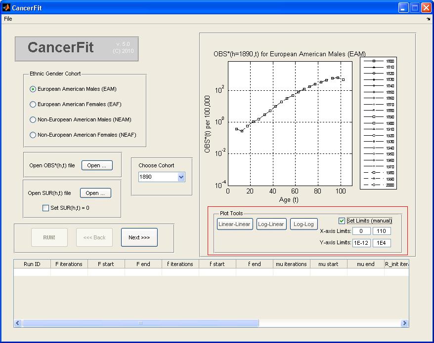
- At any point, the graph plot on the right can be converted to different scales and can also be converted into a Linear-Linear, Log-Linear and Log-Log axis scale. To set manual limits on the x and y axis of the graph plot, check the Set Limits checkbox and enter the manual x-axis and y-axis limits.
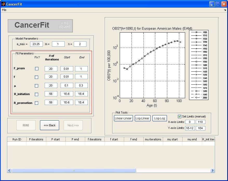
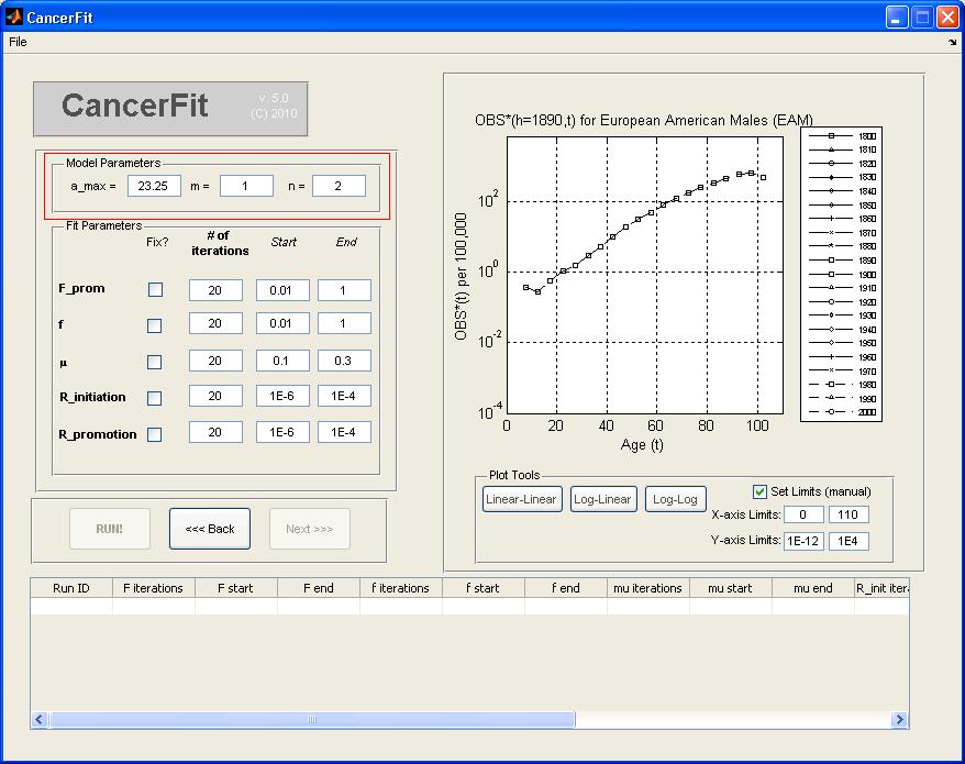
Step 4: Set up the Parameters for the CancerFit Run
- Click on the Next >> Button.
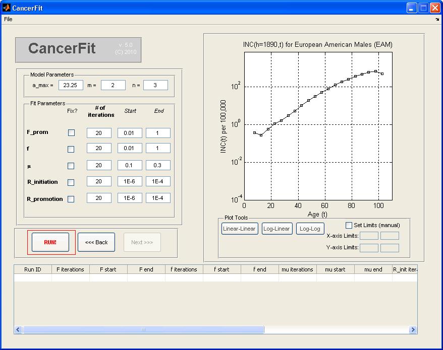
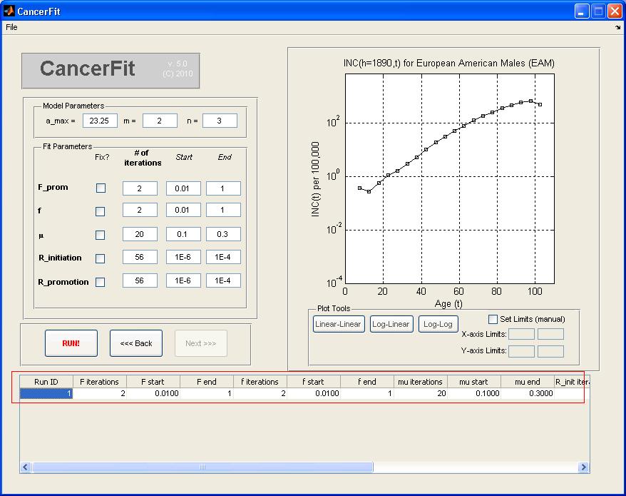
- Set the model parameters a_max, m and n. For this example, pick a_max = 23.25, m = 2, n = 3.
- Set the fit variable parameters: the number of iterations, the starting and ending values of the range of the variable.
Note, R_initiation represents the geometric mean of the initiation rates and R_promotion represents the geometric mean of all
the promotion rates. If you want to fix a variable to a specific fixed value, check the Fix? checkbox and set the
value to be fixed in the "Start" textbox. For this example, set the following parameters:
- F = 0.01 .. 1 over nF = 2 iterations
- f = 0.01 .. 1 over nf = 2 iterations
-
 = 0.10 .. 0.30 over n = 20 iterations
- Rinitiation = 1E-6 .. 1E-4 over nRij = 56 iterations
- Rpromotion = 1E-6 .. 1E-4 over nRA = 56 iterations
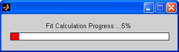
- Click on the "Run!" Button when ready to run all 20 x 20 x 20 x 56 x 56 fits. A progress bar will pop up when CancerFit is running all fits.
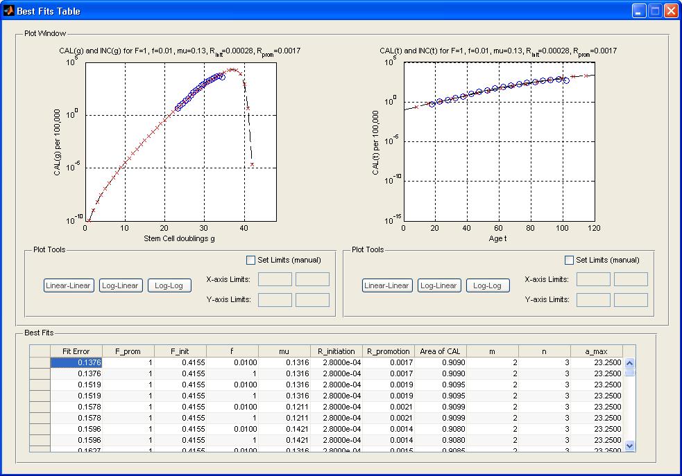
Step 5: View the CancerFit Results
- Click on the row of the table corresponding to the CancerFit run you want to view. The 10 most recent CancerFit runs can be viewed in this table. After clicking on the row to view the results, a BestFit window will popup with the top "num_fits" (which is set to 100 in the code) fits. The two graph plots will show the INC(h=1890) curve as well as the CAL(h=1890) in the "g" and "t" domain respectively. The plots can be manually adjusted into different limits and scales using the tools underneath each plot.
- Clicking on any row of the fits will update the two graph plots. Each row shows the fit error(defined in the paper), and the parameters that result in the fit.
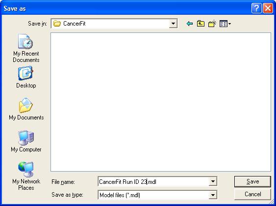
Step 6: Save the CancerFit results
- Click on the File > Save in the menu bar of the CancerFit tool. Save the file as a ".mdl" file. To open the file at a later time, run CancerFit and go to File > Open.
Step 7: Exit from CancerFit
- Close any CancerFit or BestFits windows open. No work will be saved unless you save your work using File > Save.